
Two assets can share identical expected return and identical volatility on paper and still deserve very different position sizes. The variable that changes everything is one most sizing models ignore: can you actually exit when you need to?
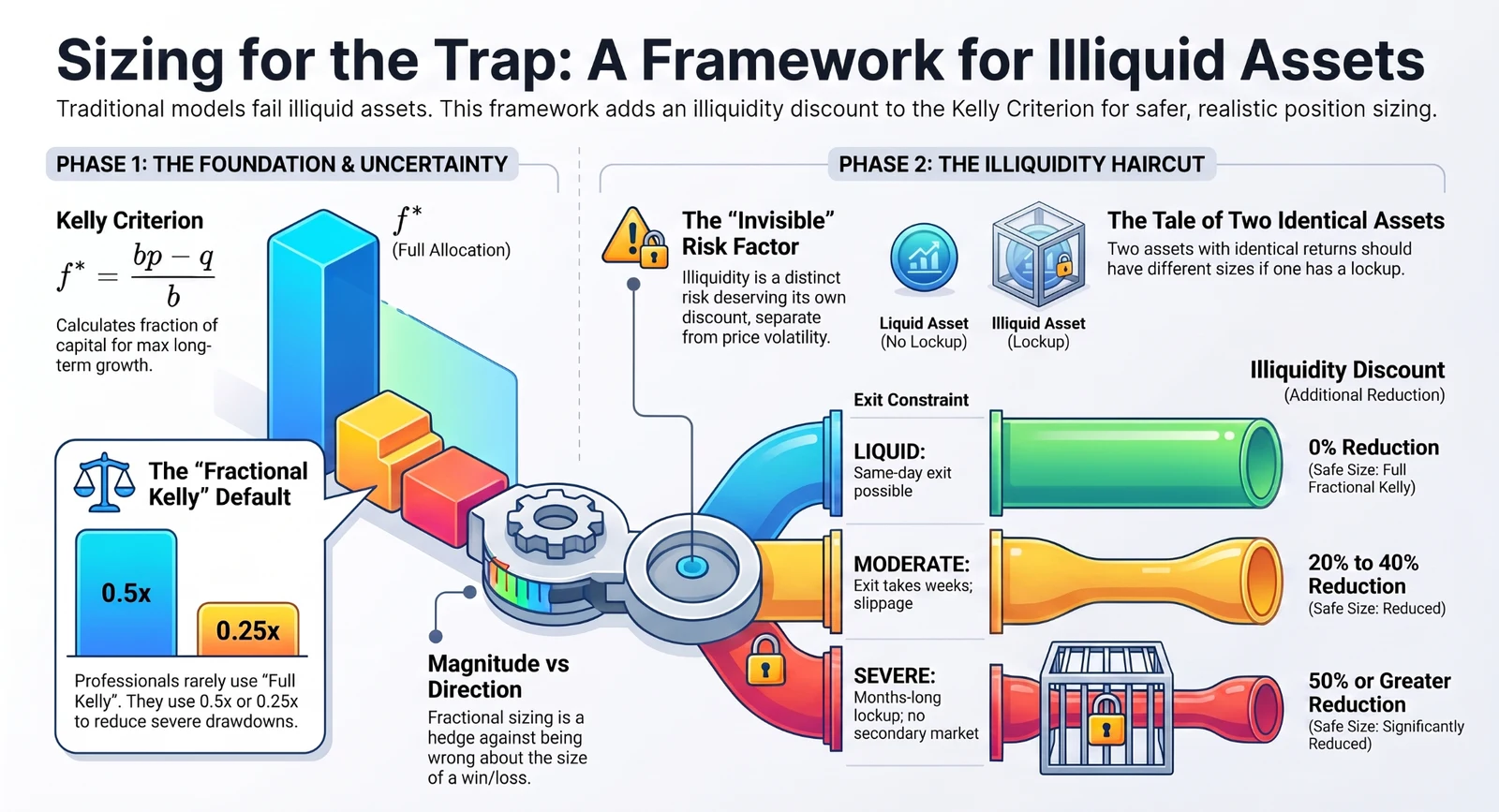
Most sizing frameworks answer the how much question using inputs like expected return and volatility (in mean-variance models) or win rates and payout ratios (in binary Kelly models), quietly assuming you can sell whenever you decide to. Traditional mean-variance models focus on expected return, volatility, and correlation, while binary Kelly models use estimated probabilities and payoff ratios. Neither basic framework automatically captures lockups and market impact.
This article uses fractional Kelly as a starting point, then applies a separate heuristic adjustment for liquidity and lockup risk. It builds on the concentration risk metrics covered earlier in this cluster, since high holder or wallet concentration directly impacts liquidity depth, creating risks of abrupt selling, price gaps, and correlated exits.
What the Kelly Criterion Actually Optimizes For
The Kelly criterion comes from outside finance entirely. John Kelly derived it in a 1956 Bell Labs paper about transmitting information over a noisy communication channel, not about markets. Edward Thorp later carried the same math into blackjack, then into securities trading, which is how it ended up as a position-sizing tool.
The formula in its simplest binary form (assuming a fixed horizon and a 100% loss upon failure) is
f* = (bp - q) / b,
where p is the probability of a favorable outcome, q is the probability of an unfavorable one (1 - p), and b is the net payout ratio (net gain per dollar wagered if you win). The output, f*, is the fraction of capital to allocate.
The basic binary Kelly formula assumes known probabilities, known gains on wins, and a known loss outcome (such as a 100% total loss) over a specific time horizon. In private-market and crypto assets, downside outcomes are rarely a standardized 100% loss; they range from partial recovery and temporary drawdowns to complete illiquid defaults over varying investment horizons.
What Kelly actually maximizes is the long-run geometric growth rate of capital, not the expected value of any single bet. That distinction matters more than it sounds. A bet with positive expected value can still be a bad idea to size heavily if it carries enough variance to wipe out a large share of capital along the way, since a large enough drawdown requires a disproportionately larger gain just to recover. Kelly sizing accounts for that compounding effect directly.
Why Full Kelly Is Rarely Used in Practice
The full Kelly fraction assumes your probability and payout estimates are exactly correct. In real markets, they never are. Even small errors in estimating p can push the optimal fraction well past what's actually safe, and full Kelly portfolios are documented to produce severe, uncomfortable drawdowns even when the underlying edge is real. This is why the practitioner standard isn't full Kelly at all; it's a fraction of it.
Half-Kelly or quarter-Kelly sizing, betting 50% or 25% of what the formula technically recommends, is a commonly discussed practical adjustment. Fractional Kelly can reduce the damage caused by estimation error, but it does not validate or solve the underlying probability and payoff assumptions
Kelly Fraction | Typical Use Case | Trade-off |
Full Kelly (1.0x) | Theoretical benchmarking | Maximizes theoretical growth, produces severe drawdowns |
Half-Kelly (0.5x) | Commonly discussed practical adjustment | Meaningfully smaller drawdowns, modest growth-rate cost |
Quarter-Kelly (0.25x) or lower | High parameter uncertainty, tail risk, or model instability | Conservative; chosen based on probability error, correlation, and drawdown tolerance |
The lower the confidence in your own probability and payout estimates, the smaller the fraction should be. This isn't a hedge against being wrong about direction but being wrong about magnitude, which is the input Kelly sizing is most sensitive to.
Why Illiquidity Changes The Math, Not Just The Label
Basic Kelly models do not automatically capture long lockups, uncertain exit prices, market impact or the inability to rebalance when assumptions change.
Academic research on portfolio choice with illiquid assets, published as an NBER working paper by Ang, Papanikolaou, and Westerfield, supports treating illiquidity as a separate portfolio constraint. Their modeling shows that the cost of illiquidity is highest for risk-averse investors with limited portfolio flexibility. It depends on how much flexibility the rest of the portfolio actually has. (Note that while this research supports an explicit constraint, it does not prescribe specific percentage haircut schedules).
Separately, research on asset pricing in illiquid markets by Francis Longstaff analyzed trading restrictions. In some modeled scenarios, Longstaff found very large welfare costs from trading restrictions, illustrating that illiquidity can have substantial economic value.
Building an Illiquidity Discount Into the Kelly Fraction
The practical adjustment is to treat illiquidity as a second, separate haircut applied after the standard fractional Kelly calculation, not folded into the volatility estimate. A simple framework:
- Calculate the base Kelly fraction using time-horizon-consistent probability and payout estimates.
- Apply a fractional Kelly adjustment (such as 0.5x or 0.25x) for parameter uncertainty.
- Apply a further illiquidity discount based on comprehensive exit constraints. Exit time is only one variable; liquidity evaluation must also consider order-book depth, DEX liquidity, expected slippage, daily volume, position size relative to market depth, lockup terms, redemption gates, and counterparty risks.
The adjustment bands below are illustrative heuristics, not empirically validated universal discounts:
Exit Constraint | Additional Illiquidity Discount (Heuristic) |
Liquid, same-day exit with minimal market impact | None |
Moderate constraint (days to weeks, order-book depth constraints, moderate slippage) | 20% to 40% reduction on fractional Kelly size |
Severe constraint (lockup in months, thin DEX/order-book liquidity, transfer restrictions) | 50% or greater reduction on fractional Kelly size |
A Multi-Constraint Worked Example
Consider an asset evaluated over a 12-month horizon with a 55% probability of a successful outcome (p = 0.55, q = 0.45) yielding a net 1.5x payout ratio (b = 1.5), assuming a 100% loss on failure.
- Raw Kelly Fraction: f* = (1.5 * 0.55 - 0.45) / 1.5 = 25%.
- Fractional Kelly Adjustment: Applying a half-Kelly adjustment (0.5x) for estimation error yields 12.5%.
- Illiquidity Discount: Applying a 50% heuristic discount for a 6-month lockup and thin secondary liquidity brings the model output to 6.25%.
However, Kelly output should serve as a starting point, not the final allocation. Independent portfolio limits must be overlaid to establish maximum ceilings:
Constraint / Limit Type | Calculated / Permitted Cap |
Half-Kelly & Illiquidity-Adjusted Model Output | 6.25% |
Market Volume & Exit-Capacity Limit | 4.0% |
Total Illiquid Exposure Budget Cap | 5.0% |
Single-Issuer / Asset Ceiling | 3.0% |
Final Recommended Position Ceiling | 3.0% |
Bottom Line
Kelly-criterion logic gives you a mathematically grounded starting point for position sizing, but the raw formula alone was never built for assets you can't exit on demand. Fractional Kelly addresses estimation uncertainty. A separate illiquidity discount addresses the risk of being trapped in a losing or oversized position with no way out. Both haircuts belong in the calculation, and skipping either one means the optimal position size on paper is larger than what's actually safe to hold.
Frequently Asked Questions
Where do the probability and payout numbers in the Kelly formula actually come from?
Due-diligence findings (such as audit reports, tokenomics scoring, and concentration metrics) can inform potential scenario analysis, but they should not be converted directly into numerical probabilities unless the mapping has been calibrated and validated.
For uncertain crypto and private assets, multi-scenario probability distributions (e.g., total loss, base case, exceptional outcome) combined with stress testing provide a far more defensible input structure than arbitrary binary assignments. Both probability and payout inputs must also be aligned to the exact same time horizon.
Does Kelly sizing work the same way when you're allocating across a whole portfolio, not just one position?
Not directly. Multi-position allocations must address correlation and common factor risks early. Private market and crypto holdings often share underlying market beta, liquidity providers, custodians, funding environments, and unlock cycles. Holding multiple small, highly correlated positions creates a single concentrated risk factor. Portfolio-level Kelly logic sizes assets relative to their joint variance-covariance contribution rather than sizing them in isolation.
How often should a position sized this way be reviewed and adjusted?
Positions should be monitored through a combination of periodic scheduled reviews and event-driven reviews. Key triggers requiring immediate re-evaluation include protocol upgrades, vesting/unlock events, funding rounds, regulatory updates, liquidity changes, custodian shifts, or thesis breaches.
Disclaimer: This article is for educational purposes only and is not financial or investment advice. Position-sizing models rely on probability and payout estimates that are inherently uncertain, and past illiquidity premium data does not guarantee future compensation for holding illiquid assets.