
A 2026 preprint examining tokenized real-world assets constructed its empirical analysis from only 54 token-month observations. The dataset covered nine Ethereum-based assets over the six-month period from December 2025 to May 2026. Even this limited sample required careful interpretation because recorded on-chain transfers could represent minting, redemptions, treasury movements, custodial rebalancing, or genuine secondary-market transactions. Therefore, transfer volume was treated as a proxy for observed activity rather than a direct measure of market depth or execution quality.
This example illustrates a broader private-market problem: the visible number of records can be much larger than the economically usable sample. A database may appear extensive, but the available evidence shrinks after duplicate entities, immature outcomes, stale valuations, inconsistent identifiers, and information unavailable at the original decision date are removed.
The remaining companies may also belong to the same investment vintage, sector, geography, or economic cycle. Consequently, those records may be correlated rather than fully independent observations.
These limitations explain why machine-learning models for illiquid assets face distinct constraints. They cannot rely on the frequent prices, synchronized timestamps, mature labels, and comparatively stable relationships available in public markets.
The central problem is not simply whether a dataset contains enough rows. The more important question is whether those rows provide independent, point-in-time evidence capable of supporting a reliable investment prediction.
So, how do small-N, non-stationary private-market datasets break familiar machine-learning assumptions, and which technical controls are needed before their predictions can support investment decisions?
Data Sparsity Is More Than Missing Rows
Private-market sparsity appears in several forms. A database can contain thousands of rows, yet several may describe one company across funding rounds. Deals from the same sector and vintage may also share one capital and exit regime.
As a result, row count should never be treated as equivalent to sample size. Entity count, outcome maturity, clustering, and decision-time availability must also be considered.
Outcomes are delayed. A company screened in 2024 may still be operating in 2026, so labeling it a failure would be wrong. Its outcome is right-censored because the observation window ended before the event.
This distinction matters because unresolved observations are not negative observations. A company that has not yet raised another round, exited, defaulted, or shut down may simply require a longer observation window.
Missingness is selective. Revenue may be absent because the company is pre-revenue, management declined to disclose it, or the data vendor never captured it. Treating all three cases as zero creates a false signal.
Reported valuations are irregular, changing mainly after an appraisal, financing, impairment, or secondary transaction. Failed and rejected opportunities are also easier to lose than successful ones.
Data property | Public markets | Private markets | Modeling consequence |
Observation frequency | Daily or intraday | Quarterly or event-driven | Irregular time steps |
Price formation | Continuous trading | Appraisal or transaction | Stable target values |
Outcome maturity | Often rapid | Frequently measured over years | Censored labels |
Missingness | More standardized | Often selective | Biased imputation |
Cross-sectional scale | Large universe | Small stage-specific cohorts | High estimator variance |
Transaction costs | Usually observable and comparatively low | Negotiated, uncertain, and potentially substantial | Predicted value may not be executable |
Historical revisions | Usually limited to traded prices | Valuations and company records may be revised later | Backtest results may change when data is refreshed |
The effective sample size is therefore smaller than the visible row count. Ten companies from one 2021 software cohort do not provide ten fully independent economic observations if the same funding boom shaped all of them.
The missingness mechanism also matters. Data can be missing completely at random, missing at random after conditioning on observed variables, or missing not at random. Private-market financial fields often fall into the third category because disclosure itself may relate to company quality, bargaining power, distress, or fundraising strategy.
As a result, routine median imputation can preserve the table while corrupting the economic meaning of the feature.
Public-Market Assumptions Break in Illiquid Assets
Many public-market ML workflows rely on frequent observations, synchronized timestamps, price discovery, and relationships that remain stable long enough to estimate. Private markets weaken each assumption.
Weak stationarity requires stable means, variances, and dependence structures. Ergodicity requires observations over time to represent the wider process. Venture vintages often behave like separate regimes because rates, exits, valuations, and capital supply change.
Kaplan and Schoar found large performance differences across private-equity funds and cyclical market entry. Funds formed during boom periods were less likely to raise follow-on funds, supporting explicit vintage controls rather than one pooled distribution.
A feature can therefore reverse meaning. Rapid hiring may indicate demand in one cycle and poor cost discipline in another. Fast fundraising may signal external confidence during a selective market but speculative excess when capital is abundant.
Random cross-validation hides this shift. A shuffled split can train on 2022 deals and test on 2018 deals. The model is then evaluated on the past after learning relationships from a later financing environment.
A stronger design trains on older vintages, tunes only inside that historical window, and tests once on a later vintage with mature outcomes. Rolling-origin validation shows how performance changes as the decision date moves forward. Leave-one-vintage-out testing reveals whether one unusually favorable cohort drives the result.
n = creates another break.
neff= effective number of independent observations
As p approaches, neff coefficients become unstable, variable importance changes across resamples, and small data revisions can alter the selected model.
The sample covariance matrix is:
Σ^=1 / n−1 XT X
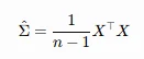
It may become singular or poorly conditioned when the feature dimension is large relative to sample size. Ledoit and Wolf introduced a shrinkage estimator that combines the sample covariance matrix with a structured target, improving invertibility and stability.
A deeper model is therefore not automatically better. A 2024 benchmark of more than 300 tabular datasets compared 32 deep and tree-based methods and found that rankings varied with dataset characteristics. Architecture choice must follow matched testing rather than assumed superiority.
For small-N financial machine learning, model capacity must be earned through later-vintage evidence. A regularized logistic model that remains calibrated may be more useful than a neural network that produces a higher historical AUC but unstable live probabilities.
Illiquidity Changes Labels, Risk, and Validation
Illiquidity changes what the model observes. Latent economic value, reported appraisal value, observed transaction price, and executable secondary-market price can diverge for long periods.
When appraisals remain unchanged between reporting dates, the return series appears smoother than the underlying exposure. A company can deteriorate economically while its recorded mark remains flat until the next financing event or impairment.
Getmansky, Lo, and Makarov showed that illiquidity can create serial correlation, understate volatility, and inflate measures such as the Sharpe ratio. Their analysis used 908 hedge funds, so it is a methodological analogue rather than a direct private-equity estimate.
The dataset must therefore store valuation age, mark type, source, and time since the last arm’s-length price. A financing-round valuation should not be treated as equivalent to an executable secondary sale. Likewise, an internal manager mark should remain distinguishable from an independent appraisal.
Long appraisal gaps may require state-space or latent-value models. However, these methods estimate an unobserved process; they do not convert a stale mark into a verified market price.
Label construction is equally difficult. Follow-on funding, acquisition, shutdown, default, realized return, and secondary liquidity are different targets. A company that raises another round is not automatically a profitable investment. An acquisition may represent either a successful exit or a distressed sale.
Cochrane showed how selection changes venture-capital estimates. Before adjustment, the mean log return in his sample was about 100%. After correcting for selection, it fell to about 7%, while volatility remained near 100%. These historical estimates show how strongly the observation process can distort labels.
Unresolved cases should therefore remain separate from negative outcomes. Survival models can estimate time to financing, failure, or exit while accounting for right censoring. A fixed-horizon classifier may also work, but every company must receive the same observation window.
A 2025 private-asset allocation preprint models several constraints often absent from public-market systems, including illiquidity, delays between commitments, capital calls and distributions, time-varying business cycles, and serial correlation in reported returns.
For tokenized real-world assets, on-chain activity does not remove the problem. A 2026 preprint found substantial liquidity differences across Treasury-backed, gold-backed, and private-credit-related tokens, while asset value alone did not reliably predict observed liquidity. Tokenization creates transfer records, not guaranteed secondary demand.
Therefore, a model has millions of wallet events. But only a small number of meaningful redemptions, defaults, price-forming trades, or completed liquidation outcomes.
A Defensible Architecture for Sparse Private-Market ML
A reliable pipeline starts with point-in-time evidence. Each record should include an entity identifier, event date, publication date, screening cutoff, vintage, mark type, label status, and outcome deadline. Otherwise, current information can leak into historical tests.
The model ladder should begin with a stage-and-sector base rate. Next come regularized logistic or ridge regression, hierarchical Bayesian models, and survival models for censored outcomes. Constrained gradient boosting may follow.
An ensemble should enter production only if it improves a later, untouched vintage and the gain survives uncertainty testing.
The workflow should follow this sequence:
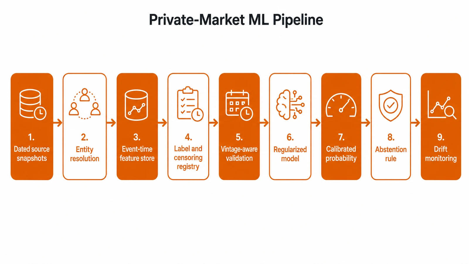
Entity resolution comes early because one company may appear under several names, subsidiaries, legal entities, or wallet addresses. Incorrect joins can create duplicate outcomes or allow information from related entities to cross the screening cutoff.
Validation should use rolling-origin or leave-one-vintage-out splits. Hyperparameter tuning must remain inside the training window. Where labels overlap across time, overlapping observations should be purged and an embargo placed before the test period.
Performance reporting must match the decision. Use precision at K when only the top K deals can be reviewed. Report PR-AUC beside the positive-class rate. Use the Brier score and calibration slope for probability forecasts. Apply concordance or time-dependent metrics for survival outcomes.
Point estimates are not enough. A 2025 asset-pricing preprint developed confidence intervals and bootstrap procedures for machine-learning forecasts, reinforcing the need to show uncertainty rather than only a score.
An abstention rule is equally important. If critical fields are missing, the company lies outside the training distribution, or source records conflict, the system should return insufficient evidence rather than a precise probability.
Synthetic data may test pipelines, privacy controls, or rare-event scenarios. It cannot create independent evidence of exits, defaults, redemptions, or executable liquidity.
Deployment Controls for Institutional Use
Before a model influences capital allocation, the review team should confirm that:
- The target event and prediction horizon are explicit.
- neff is reported by entity, vintage, and outcome maturity.
- Every feature existed at the original screening date.
- Failed, rejected, delisted, and unresolved cases remain in the dataset.
- The model beats base-rate and regularized benchmarks.
- The newest mature vintage stayed untouched during selection.
- Probabilities are calibrated and the system can abstain.
- A defined drift threshold triggers recalibration or suspension.
These controls fit within robust model validation architectures for algorithmic deal screening. Replace the working-document address with the final canonical page before publication.
FAQs
Why do public-market ML models fail in private markets?
They may fail because private-market observations are small in number, irregular, stale, selected, and dependent on vintage conditions. Random splits, synchronized prices, and stable feature relationships become unreliable assumptions.
Which models work best with small-N private-market data?
Regularized regression, hierarchical Bayesian models, survival analysis, and constrained tree methods are strong starting points. The best choice depends on the target, feature count, censoring structure, and number of independent vintages.
Can more features solve private-market data sparsity?
Usually not. When p grows faster than neff, variance rises and feature selection becomes unstable. New variables help only when they add point-in-time information that survives later-vintage testing.
How should stale valuations be handled?
Track valuation age and mark type, separate appraisals from transaction prices, test for serial correlation, and use latent-value or de-smoothing methods only when their assumptions match the reporting process.
Data sparsity is the evidence problem. Different model constraints are the consequence. In illiquid assets, reliable machine learning requires smaller models, stricter chronology, explicit censoring, uncertainty estimates, and the discipline to refuse a prediction when the data cannot support one.